通常為了模型能更好的收斂,隨着訓練的進行,希望能夠減小學習率,以使得模型能夠更好地收斂,找到loss最低的那個點.
tensorflow中提供了多種學習率的調整方式.在搜索decay.可以看到有多種學習率的衰減策略.
- cosine_decay
- exponential_decay
- inverse_time_decay
- linear_cosine_decay
- natural_exp_decay
- noisy_linear_cosine_decay
- polynomial_decay
本文介紹兩種學習率衰減策略,指數衰減和多項式衰減.
- 指數衰減
tf.compat.v1.train.exponential_decay(
    learning_rate,
    global_step,
    decay_steps,
    decay_rate,
    staircase=False,
    name=None
)
learning_rate 初始學習率
global_step 當前總共訓練多少個迭代
decay_steps 每xxx steps后變更一次學習率
decay_rate 用以計算變更后的學習率
staircase: global_step/decay_steps的結果是float型還是向下取整
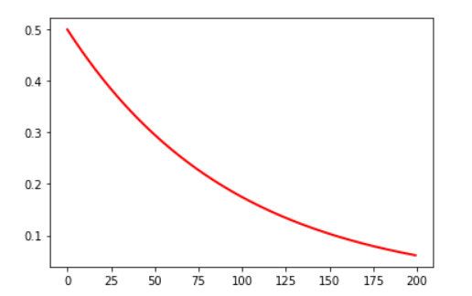
學習率的計算公式為:decayed_learning_rate = learning_rate * decay_rate ^ (global_step / decay_steps)
我們用一段測試代碼來繪製一下學習率的變化情況.
#coding=utf-8
import matplotlib.pyplot as plt
import tensorflow as tf

x=[]
y=[]
N = 200 #總共訓練200個迭代

num_epoch = tf.Variable(0, name='global_step', trainable=False)
with tf.Session() as sess:
    sess.run(tf.global_variables_initializer())
    for num_epoch in range(N):
        ##初始學習率0.5,每10個迭代更新一次學習率.
        learing_rate_decay = tf.train.exponential_decay(learning_rate=0.5, global_step=num_epoch, decay_steps=10, decay_rate=0.9, staircase=False)
        learning_rate = sess.run([learing_rate_decay])
        y.append(learning_rate)

#print(y)

x = range(N)
fig = plt.figure()
ax.set_xlabel('step')
ax.set_ylabel('learing rate')
plt.plot(x, y, 'r', linewidth=2)
plt.show()
結果如圖:
- 多項式衰減
tf.compat.v1.train.polynomial_decay(
    learning_rate,
    global_step,
    decay_steps,
    end_learning_rate=0.0001,
    power=1.0,
    cycle=False,
    name=None
)
設定一個初始學習率,一個終止學習率,然後線性衰減.cycle控制衰減到end_learning_rate后是否保持這個最小學習率不變,還是循環往複. 過小的學習率會導致收斂到局部最優解,循環往複可以一定程度上避免這個問題.
根據cycle是否為true,其計算方式不同,如下:
#coding=utf-8
import matplotlib.pyplot as plt
import tensorflow as tf

x=[]
y=[]
z=[]
N = 200 #總共訓練200個迭代

num_epoch = tf.Variable(0, name='global_step', trainable=False)
with tf.Session() as sess:
    sess.run(tf.global_variables_initializer())
    for num_epoch in range(N):
        ##初始學習率0.5,每10個迭代更新一次學習率.
        learing_rate_decay = tf.train.polynomial_decay(learning_rate=0.5, global_step=num_epoch, decay_steps=10, end_learning_rate=0.0001, cycle=False)
        learning_rate = sess.run([learing_rate_decay])
        y.append(learning_rate)

        learing_rate_decay2 = tf.train.polynomial_decay(learning_rate=0.5, global_step=num_epoch, decay_steps=10, end_learning_rate=0.0001, cycle=True)
        learning_rate2 = sess.run([learing_rate_decay2])
        z.append(learning_rate2)
#print(y)

x = range(N)
fig = plt.figure()
ax.set_xlabel('step')
ax.set_ylabel('learing rate')
plt.plot(x, y, 'r', linewidth=2)
plt.plot(x, z, 'g', linewidth=2)
plt.show()
繪圖結果如下:
cycle為false時對應紅線,學習率下降到0.0001后不再下降. cycle=true時,下降到0.0001后再突變到一個更大的值,在繼續衰減,循環往複.
在代碼里,通常通過參數去控制不同的學習率策略,例如
def _configure_learning_rate(num_samples_per_epoch, global_step):
  """Configures the learning rate.

  Args:
    num_samples_per_epoch: The number of samples in each epoch of training.
    global_step: The global_step tensor.

  Returns:
    A `Tensor` representing the learning rate.

  Raises:
    ValueError: if
  """
  # Note: when num_clones is > 1, this will actually have each clone to go
  # over each epoch FLAGS.num_epochs_per_decay times. This is different
  # behavior from sync replicas and is expected to produce different results.
  decay_steps = int(num_samples_per_epoch * FLAGS.num_epochs_per_decay /
                    FLAGS.batch_size)

  if FLAGS.sync_replicas:
    decay_steps /= FLAGS.replicas_to_aggregate

  if FLAGS.learning_rate_decay_type == 'exponential':
    return tf.train.exponential_decay(FLAGS.learning_rate,
                                      global_step,
                                      decay_steps,
                                      FLAGS.learning_rate_decay_factor,
                                      staircase=True,
                                      name='exponential_decay_learning_rate')
  elif FLAGS.learning_rate_decay_type == 'fixed':
    return tf.constant(FLAGS.learning_rate, name='fixed_learning_rate')
  elif FLAGS.learning_rate_decay_type == 'polynomial':
    return tf.train.polynomial_decay(FLAGS.learning_rate,
                                     global_step,
                                     decay_steps,
                                     FLAGS.end_learning_rate,
                                     power=1.0,
                                     cycle=False,
                                     name='polynomial_decay_learning_rate')
  else:
    raise ValueError('learning_rate_decay_type [%s] was not recognized' %
                     FLAGS.learning_rate_decay_type)
推薦一篇: 對各種學習率衰減策略描述的很詳細.並且都有配圖,可以很直觀地看到各種衰減策略下學習率變換情況.
本站聲明:網站內容來源於博客園,如有侵權,請聯繫我們,我們將及時處理
【其他文章推薦】
※專營大陸空運台灣貨物推薦
※台灣空運大陸一條龍服務